lab 8

Network analysis is a tool used in both transportation and economic geography in order to analyze the allocation and displacement of places. One aspect of displacement is shortest path analysis which finds the path with the minimum cumulative impedance between nodes on a network. With shortest path analysis, there is a node of origin, destination, and possibly other nodes that act as stops along the path. Shortest path analysis allows for routes to be created based upon the shortest distance or shortest amount of time it takes to move from the origin to the destination. Allocation involves analyzing the spatial distribution of resources throughout a network in order to establish a service area. Service areas can be established based upon a time limit or maximum distance from the node. Optimal path involves finding the route with the least amount of travel costs.
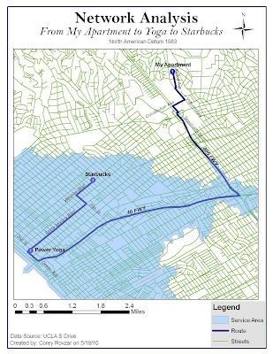
For this lab, the problems in question were 1. What is the best path to take to my yoga studio and then to Starbucks? and 2. Does the studio I go to serve the area where I live? My Thursday morning route was analyzed to find the optimal route. My route includes starting at my apartment, stopping at the yoga studio, and then ending at a Starbucks on Wilshire. Additionally, the service area for my yoga studio was generated to evaluate whether or not the studio served the area where I live. The parameters for the optimal route were kept at their default values: the impedance was time (minutes), U-turns were allowed everywhere, and the output shape type was true shape. The parameter values for time included: 10, 15, 20, 25, 30, 35, 50, and 65 miles per hour. Lastly, the search tolerance was set at 5000 meters. Setting the impedance as time generated the fastest route based on speed limits. Similarly, the service area was created using default parameters: the impedance was time with default breaks of 5, direction was away from the facility, u-turns were allowed everywhere, restrictions were one way, and the parameter values and search tolerance were the same as those used for generating the optimal route. Distance units for both were set to miles. Setting the impedance as time and default breaks for the service area to 5, resulted in a service area that was restricted to areas within 5 minutes of the studio.
According to the optimal route from my apartment to the yoga studio, it is quickest for me to take Kelton, to Veteran, to Constitution, to Sepulveda, to the 405, to the 10, to Ocean, to Santa Monica, and lastly to 2nd to end at 1410 2nd St. From the studio to Starbucks, it is quickest to take 2nd, to Santa Monica, to 20th, and finally to Wilshire to end at 2525 Wilshire Blvd. Although this route should be fastest due to a higher speed limit on the freeways, ultimately it is dependent on traffic. Depending on the time that I leave, it may be faster to take side streets due to higher congestion on the freeways. The network analysis could be improved by having the capability to analyze traffic in addition to local speed limits. The service area for the yoga studio included everything that was less than 5 minutes away. Based on these results, my apartment is more than 5 minutes away from the studio. Therefore, it could be argued that it is not practical for me to drive all the way to Santa Monica for yoga when there are closer yoga studios that serve my area. However, the network analysis only accounts for travel costs and not other factors that may make it worthwhile to travel farther. The yoga studio I go to happens to be donation-based, meaning I can pay however much I have for the class without being locked into a plan. Because of this, it is worth it for me to pay the transportation costs of time and gas money to go to Santa Monica versus paying more for the classes closer to my apartment. The results generated by the network analysis would be realistic for suburban areas and small cities that don’t experience large amounts of traffic. However, for Los Angeles and other major cities, the network analysis would only really be reliable during hours where there is minimal traffic. Adding a traffic analysis component to the network analysis would increase the accuracy of the network analysis for highly congested areas such as Los Angeles.

Lab 7- Watershed Analysis

Tibetan Plateau Watershed Analysis

Introduction:

Watershed analysis is a valuable tool that utilizes digital elevation models and raster data to delineate watersheds and define features such as stream networks and watershed basins. It is an essential device in a variety of fields including hydrology and environmental modeling. An important aspect of watershed analysis is the spatial scale in which it is performed. At a larger scale, there are fewer watersheds while at a smaller scale, more watersheds are produced. The optimal scale ultimately depends on the level of detail that best suits the sample area. Factors that influence the overall quality of the watershed analysis include the quality of the digital elevation model, the algorithm used for deriving flow directions, and the threshold used to delineate the stream network. In ArcGIS, the D8 algorithm is used because it is simple, efficient, and ideal for evaluating mountainous regions. For this lab, an area-based analysis was performed for the Tibetan Plateau with watersheds created for each stream section. Analyzing the relationship between elevation and drainage networks allows for an understanding of the location of surface water such as lakes. Generating watershed analysis provides the foundational base for further surface modeling.

Methods:

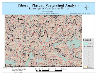
The first step in delineating watersheds involved filling in the depressions within the digital elevation model. For the fill operation, a z-limit of 15 was used because it generated the most practical watershed basins with larger lakes having their own watershed basins. A denser stream network should have more, but smaller, watersheds. Additionally, using this value created watersheds that organized around stream networks and visually, made sense. The z-limit represents the maximum elevation difference between a sink and its pour point. Only sinks that have a difference in z-values between a sink and its pour point that is less than the z-limit will be filled. Using a z-value higher than 15 generated too many watersheds, while using a z-limit lower than 15 generated too few. After the basins were delineated, flow direction was calculated according to the D8 method which is the default method for ArcGIS. This method uses the 8 surrounding cells with a weighted distance to calculate the center cells flow direction. The stream network was created using the Con tool and setting a threshold of greater than or equal to 1,000 cells. The higher the threshold was set, the less detail that the map displayed because a higher threshold value results in a less dense stream network and fewer internal watersheds. While 100, 500, and 700 threshold values were tested, ultimately a threshold of greater than or equal to 1000 seemed to generate the most accurate results with stream networks clearly visible. The final steps involved creating watershed basins, which related to the fill z-limit value, and assigning a stream order to the stream networks which was based on the default Strahler method.



Analysis:

According to the watershed map, the hydrology in the Tibetan Plateau is very extensive with many stream networks and watershed basins. As a result, a large number of lakes have formed with the largest occurring in areas with the most expansive stream networks. Additionally, many of the streams contributing to the formation of lakes have a stream order of 1 suggesting that the water is flowing from a primary source to the lake and thus, more water is able to be collected rather than being diverted to other streams.

Comparison:

By comparing my map, with the downloaded data on watersheds within the Tibetan Plateau region, it is evident that my map is more detailed and has greater accuracy. The data attained from the Global Drainage Basin Database was for all of Asia. As a result, it does not show as much detail for the Tibetan Plateau especially concerning lakes and stream networks. My map shows a much more extensive stream network as well as a greater number of lakes. However, the watershed basins appear to be very similar, suggesting that the z-limit I used when creating a fill was accurate. Other differences include that my map was based on an area-based watershed method while the downloaded data was based on a pour-point watershed method.

Comparing my stream network, basins, and lakes with a landsat image provided by the Global Land Cover suggested that most of the lakes accumulate at a medium elevation. As streams flow down mountains, ultimately most of the water will collect at a medium elevation because at a lower elevation, water has been diverted to other areas through other streams. Ultimately, comparing my generated stream networks and watershed basins with a landsat image allows for an evaluation of patterns of stream flow and lake formation as it relates to elevation.

Problems:

While digital elevation models are extremely useful for performing watershed analysis, the resolution and quality of the DEM can ultimately affect the results. A DEM with a high resolution might be too course to allow for topographic features to be shown and presents difficulty when creating a stream network. Similarly, a higher-resolution DEM might also generate smaller watershed areas compared to lower-resolution DEMs. DEMs must also be of good quality in order to allow for an accurate fill. The fill is one of the foundational steps for the analysis. Therefore, having an accurate fill will allow for greater accuracy in modeling the watershed. Ultimately, the best ways to eliminate problems with DEMs is to attain them from a reliable source and to run the watershed analysis on a variety of DEMs until accurate results are attained.

Lab 6- Georeferencing UCLA

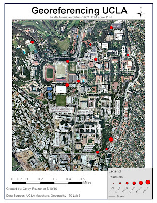
Georeferencing is an important tool that registers a map into a GIS system by applying real world coordinates. By georeferencing a map image, the map image is assigned a specific location and spatial analyses can be performed. One method to attain the real world coordinates is to utilize a GPS system which measures the coordinates based on satellite signals. Although GPS is valuable in providing coordinates, often times it is not entirely accurate due to inherent errors, user errors, and discrepancies that arise when interacting with a GIS. Overall, it is important to evaluate these uncertainties in order to minimize their effects on the georeferencing to allow for greater accuracy.
Despite its worldwide use in a variety of fields, GPS remains a relatively recent development. As a result, signal clarity and reception have not been able to be modified to produce entirely accurate results. For example, other electronic signals or structures such as walls and windows can block GPS signals and generate imprecise coordinates for a location. Additionally, limited reception in an area would result in greater difficulty for the GPS to accurately give a location’s coordinates. Another source of error when using GPS results from its use by a user. Not allowing sufficient time for the GPS to register the location as well as not remembering the exact location where the coordinates were taken ultimately results in inaccuracies. In this lab, much of the error was human-induced due to the inability to locate exactly where the coordinates were taken on a map. In order to minimize this error, it is important to use ground control points (GCP) on corners of buildings, landmarks, or easily identifiable objects that will be easy to precisely locate on a map image. Lastly, errors arise through the interaction between the GPS and GIS. Regardless of the accuracy of the GPS coordinates, matching the locations of the GCP points on the maps with the coordinates will inevitably produce some errors as it is highly unlikely that the precise location on the map will be located. In this lab, the orthophoto used was not updated and did not have a high resolution which presented some uncertainty when choosing the location where the GCP points were taken. Additionally, the points were taken by different groups who did not always report the precise the location where the coordinates were taken.
The results of these errors were represented by the GIS as residuals which provide the difference between the entered coordinates and the fitted coordinates relative to the other GCP points. Additionally, the GIS generated an RMS (root, mean, square) score which provides a measure of the overall error within the ground control points of the georeferenced map. For this lab, the georeferenced image generated an RMS of 3.39415. Some GCP points were removed when georeferencing the map due to their extremely high residual values which greatly increased the RMS. Although it is better to have a lower RMS score, ultimately human and GPS errors have generated a higher RMS value. Most of the uncertainty is likely attributed to the fact that the GCP points were collected by different groups and therefore, the exact locations of where the coordinates were taken had to be estimated on the map. Overall, I would improve the georeferencing of this image by taking the GCP points myself and in areas, such as corners of buildings, which are clearly visible and discernable on the map. Additionally, I would include ground control check points in order to check to see that my GCP points and current georeferencing were accurate.
Georeferencing is a valuable tool that allows virtually any map to be registered in space using real world coordinates. By continuing to develop greater technologies to improve GPS as well as other locational devices, greater accuracy can be attained when performing spatial analyses in GIS. Ultimately, the easiest way to minimize error within georeferencing is to control for human-induced error and be as precise as possible when measuring GCP points as well as finding the location of the GCP points on the map.