
Interpolation is the process by which unknown values in a dataset are predicted based upon known samples. It employs the principle of spatial autocorrelation in order to determine the interrelatedness between points, and if there is interrelatedness, it will determine whether or not there is a spatial pattern. Two types of interpolation include Inverse Distance Weighting (IDW) and Kriging. IDW is a deterministic technique that involves using a linear-weighted combination set of sample points in order to interpolate unknown values. Known points closer to the interpolated value will have greater weight, wheareas those farther will have less weight. Overall, this method is beneficial when a data set consists of many samples that capture the extent of local surface variation. In contrast, Kriging is a statistical interpolation technique that considers the distance and direction between sample points in order to evaluate interrelatedness between points and determine surface variations. A weighted average technique is used to measure relatedness between sample points and interpolate unknown values. A fixed or variable search radius is used to predict values and the surface does not pass through any of the points.
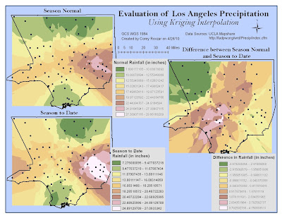
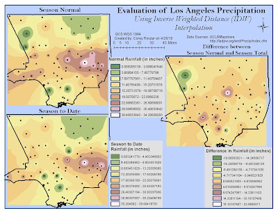
For this lab, precipitation levels for Los Angeles County were evaluated through interpolation by considering the normal precipitation levels and total season-to-date levels that were measured at various rain gauges. Both IDW and Kriging were conducted using the given parameters by ArcGIS. Based on the season normal and season total values for both interpolation maps, is evident that the highest amounts of rainfall occur in south-eastern Los Angeles while the lowest amounts are found in the far north and southern areas. However, the IDW and Kriging methods generate varying results when evaluating the difference in precipitation levels between the season normal and season total. In the IDW map, this season’s precipitation levels appear to be about average compared with the season normal, with only a few areas of either higher than average or lower than average precipitation. In contrast, the Kriging method generated more variable results with this season’s precipitation levels being greatly below average in the northwest, slightly above average centrally, and about equal to the average in the east of Los Angeles. Both interpolation methods produced surprising results because this year is an El Nino year; therefore, it is expected that there be higher than normal precipitation levels. However, the maps suggest that overall, this season’s rainfall has not been significantly higher than normal. It is important to consider that the season normal includes precipitation values from extreme El Nino years that might include unusually high values that may cause the season normal values to be skewed higher.
I believe that IDW is the best method for interpolating precipitation values for the season normal, season total, and the difference between the season normal and total because there are a significant number of sample points and precipitation does not normally vary significantly from nearby areas. Therefore, areas closest to an interpolated value are most likely to better estimate rainfall for that area and should have greater weight. Additionally, IDW interpolation passes through all the sample points, allowing for the points to influence the interpolated values, whereas Kriging does not. Kriging would not be as accurate because the spatially correlated distance and directional bias for the data set are not known. However, Kriging would be an optimal choice if we wanted to estimate error and the level of uncertainty within the interpolation. Splining would be the last method I would use for the interpolation because it creates smooth surfaces when connecting the points, and as a result, can be misleading depending on the distance between points. For this lab, splining produced negative values for both the season normal and season total precipitation levels. Because rainfall values cannot be negative, this interpolation would be confusing to a person with no understanding of the splining technique. Overall, each method has both positives and negatives. By manipulating the parameters, different patterns will be shown. Ultimately, it is up to the GIS user to decide which method is relevant to the study topic and generates spatial patterns that best simulate reality.
No comments:
Post a Comment